Build the future with machine learning

ADVERTISEMENT
Table of Contents
- Introduction
- Contents
- Preliminaries
- Data exploration
- TensorBoard setup
- Graph construction
- Create data input tensors
- Create the first convolutional layer
- Create the first downsampling layer
- Create the second convolutional layer
- Create the second downsampling layer
- Create the first dense layer
- Dropout
- Create the second dense layer
- Graph Execution
- TensorBoard visualization
- Conclusion
Introduction
In a recent post, we explored an introduction into Machine Learning purely from a theoretical perspective. Let's take a different approach, a more practical approach. This will be for those who are keen to improve their Machine Learning skills in the real-world. So what will we build? Hmmm.. let's build a Convolutional Neural Network (CNN). The Neural Network will be multi-layered, and we will use Python and Google's open-source library, "Tensorflow".
We’ll be using the MNIST dataset as we can train our model without the need of a GPU. What is MNIST? It is an image database filled with hand-written digits.
Ok... Let's build a simple two layer convolutional neural network, with maxpooling, dropout, and a couple of fully connected layers. We will also set up a log directory where we can catch log data from both the training and validation sets. This will help us monitor the performance graphically (using TensorBoard), rather than with plain old print statements.
Contents
- Preliminaries
- Data Exploration
- TensorBoard Setup
- Graph Construction
- Graph Execution
- TensorBoard Visualization
- Conclusion
Preliminaries
Python version 3.6 - Python can be found here TensorFlow version 1.1.0 - you can install Tensorflow here
Import the following libraries:
import os
import numpy as np
import tensorflow as tf
import matplotlib.pyplot as plt
Data exploration
TensorFlow makes it real simple to obtain the MNIST dataset - just import the input_data and call the method read_data_sets.
# import MNIST data
from tensorflow.examples.tutorials.mnist import input_data

mnist = input_data.read_data_sets("MNIST_data/", one_hot=True)
Let's explore the 'mnist' object under the microscope and see what is inside it...
# We see that it's a Datasets type, which makes sense
type(mnist)

# Let's check the last 5 methods that can be called on this object
dir(mnist)[-5:]
dir(mnist.train)[-5:]
Images are typically stored as a two-dimensional array of pixels per channel. The MNIST dataset has only one channel, hence why there is no colour. Below we see that there are 55,000 images in the training set, but each image is represented as a vector of length 784. This length represents the flattened version of a 28x28 pixel image.
mnist.train.images.shape
# Out: (55000, 784)
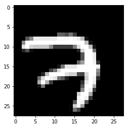
To view an image, we must first convert it back into matrix form. We do this using numpy's reshape method. Reshape the image into its original 28x28 form, then display the image in black and white using the cmap='gray' option. Notice below the numbers and tick marks on the x and y axes, showing our notion of the 28x28 pixel size of each image.
# Let's see an example of an image in the training set
plt.imshow(mnist.train.images[0].reshape((28, 28)), cmap='gray')
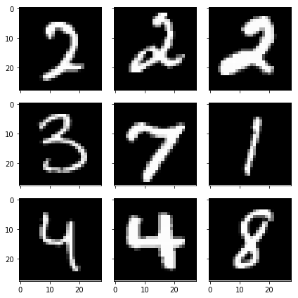
Ok still with me? let's now write a function to make it easier to sample a few images at a time, displaying them in a 3x3 grid. This makes sampling a faster process.
def show_grid_3x3(images):
   """
   Display a 3x3 grid of 9 randomly sampled numpy array images.
   : images: A batch of image data. Numpy array with shape (batch_size, 28, 28, 1)
   """
   plt.rcParams['figure.figsize'] = 6, 6
   fig, axes = plt.subplots(nrows=3, ncols=3, sharex=True, sharey=True)
   rand_idx = np.random.choice(images.shape[0], 9, replace=False) # get 5 random indices
   images = images[rand_idx]
   for i in range(3):
       for j in range(3):
           axes[i, j].imshow(images[i + 3*j].reshape((28, 28)), cmap='gray')
           plt.tight_layout()
Cool, now let's call the show_grid_3x3 function on the training set:
show_grid_3x3(mnist.train.images)
TensorBoard setup
We'll use TensorBoard to visualize several aspects of our neural network, such as the distribution of the weights and biases over time, the classification accuracy of the training and validation sets, and the computational graph. Also, we need to create a log file directory for when the neural network starts running.
Now we are going to write a function to create a directory path with a time-stamp. We wouldn't want TensorFlow overwriting our previous logs every time we run the code.
# For logging
from datetime import datetime

def logdir_timestamp(root_logdir="tf_logs"):
   """Return a string with a timestamp to use as the log directory for TensorBoard."""
   now = datetime.utcnow().strftime("%Y%m%d_%H%M%S")
   return os.path.join(root_logdir, "run-{}/".format(now))

logdir = logdir_timestamp()
We may now run TensorBoard and instruct it to monitor the directory named tf_logs:
mkdir tf_logs
tensorboard --logdir=tf_logs
Navigate to localhost:6006 in your web browser to view the TensorBoard console.
Feel free to have a look around, but there won't be anything there until we use a FileWriter to write some data to disk while the neural network is running.
Graph construction
In Tensorflow, we must first construct a graph. At this stage, we lay down the blueprint for our neural network, but no actual operations are being executed. Once the graph is complete, we will create a TensorFlow session where we can execute the operations defined in the graph.
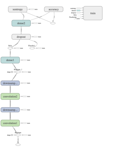
Let's have a look at what the graph should look like when we are done. We'll step through one layer at a time, starting from the bottom, where X is reshaped and fed into the convolutiona1 layer.
Create data input tensors
The first step is to create placeholders for the data to feed into the graph. We'll create a variable X to represent a batch of images, and the variable y_ to represent the corresponding labels for each image. Notice that we expect the input as a flattened vector, because that is the form in which we obtained the MNIST data. But since we are performing convolutions in this neural network, we would like to retain the two-dimensional spatial structure in the image data, so we reshape X and assigned it to the variable X_image.
Shown below are the two methods returning placeholders for the graph:
def neural_net_image_input(image_shape):
   """Constructs a tensor for a batch of image input
   image_shape: Shape of the images as a list-like object
   return: Tensor for image input
   """
   shape = None, *image_shape
   return tf.placeholder(tf.float32,
                         shape=shape,
                         name="X")

def neural_net_label_input(n_classes):
   """Constructs a tensor for a batch of label input
   n_classes: Number of classes
   return: Tensor for label input
   """
   shape = None, n_classes
   return tf.placeholder(tf.float32,
                         shape=shape,
                         name="y")
Below we input the length 784 into the Neural Network (NN), remember this is the length of the flattened image vector. The labels, denoted by the placeholder y_, has a shape of 10 as there are ten different digits to be classified in the dataset. When creating a placeholder, we use the value None to indicate an arbitrarily sized batch of images or labels.
X = neural_net_image_input([784])
y_ = neural_net_label_input(10)
X_image = tf.reshape(X, [-1, 28, 28, 1]) #  rehaped to [batch_size, rows, cols, channels]
Create the first convolutional layer
We can now write a function to create a convolutional layer since we'll be repeating this step to create another layer.
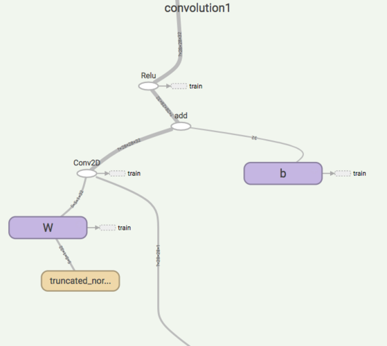
We initialize the weights by sampling from a truncated normal distribution with a standard deviation of 0.1. A truncated normal distribution is similar to a normal distribution, but if a weight is more than two standard deviations away from the mean, it is dropped and picked. We hard-code the filter (also called a kernel) to have a size of 5x5. See this for a visualization of how convolutional filters work. In the first layer, we input a single image, so the size_in variable is set to 1. size_out is the number of convolutional filters we want to create; in this case 32. The size of the filter and the number of filters are hyper-parameters we can experiment with, in an effort to improve performance - the current values are by no means optimal!
The image placeholder and the newly initialized weights are passed into the tf.nn.conv2d TensorFlow library function. To learn more about strides and padding, please refer to the TensorFlow documentation.
tf.nn.relu is another TensorFlow library function which is applied to the result of the conv2d operation. ReLU is an abbreviation for rectified linear unit, which returns the value of its argument or 0, whichever is greater.
def convolution_layer(inp, size_in, size_out, name="convolution"):
   """Creates a convolutional layer with filter of size 5x5, and size_out number of filters.
   Applies stride of [1, 1, 1, 1] with SAME padding, and appies ReLU activation.
   No downsampling within this layer - returns tensor with activation function applied only
   """
   with tf.name_scope(name):
       # Hard code convolutional filter of size 5x5
       W = tf.Variable(tf.truncated_normal([5, 5, size_in, size_out], stddev=0.1), name="W")
       b = tf.Variable(tf.constant(0.1, shape=[size_out]), name="b")
       conv = tf.nn.conv2d(inp, W, strides=[1, 1, 1, 1], padding='SAME')
       act = tf.nn.relu(conv + b)
       tf.summary.histogram("weights", W)
       tf.summary.histogram("biases", b)
       tf.summary.histogram("activations", act)
       return act
Turning to the TensorFlow graph, let's look at what is actually happening inside the first convolutional layer. The graph appears to show a fairly straightforward representation of the code...
Assign the output of the convolution_layer function to a variable named act1. This will be used as the input for the next layer.
act1 = convolution_layer(X_image, 1, 32, "convolution1")
Create the first downsampling layer
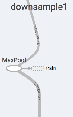
The output of the convolution layer is downsampled using maxpooling with a kernel of size 2x2. This means that the maximum value is taken for every 2x2 region of the input. This reduces the spatial size of the input, effectively reducing the number of parameters in the network and thereby reducing computational complexity and the propensity to overfit. We'll return to the topic of overfitting when we discuss the TensorBoard graphs showing the training and validation set accuracies.
def downsample_layer(act, name="maxpooling"):
   """Creates downsampling layer by applying maxpooling with hardcode kernel size
   [1, 2, 2, 1] and strides [1, 2, 2, 1] with SAME padding.
   """
   with tf.name_scope(name):
       return tf.nn.max_pool(act, ksize=[1, 2, 2, 1], strides=[1, 2, 2, 1], padding='SAME')
Notice below how the number of parameters are reduced after the maxpool operation - from 28x28 to 14x14.
Store the output of the downsampling layer in the variable h_pool1.
h_pool1 = downsample_layer(act1, "downsample1")
Create the second convolutional layer
The structure of the second convolutional layer is identical to the first one. It might be hard to see below, but notice the size of the tensors coming in, and the tensors going out - 14x14x32 to 14x14x64.
This time, set the input size to 32, and create 64 convolutional filters.
act2 = convolution_layer(h_pool1, 32, 64, "convolution2")
Create the second downsampling layer
Once again, notice the shape of the outgoing tensor. We would like to flatten this tensor into a vector, so that we can connect every single neuron together in the dense layer, a.k.a a fully connected layer. This is the reason for the 7*7*64 value for the reshape operation - the input is a 7x7x64 tensor which will then be converted into a vector of length 7*7*64=3136. The same value is then passed into the dense_layer method to create tensors of weights and biases sized appropriately.
h_pool2 = downsample_layer(act2, "downsample2")
Create the first dense layer
The dense layer performs a simple matrix multiplication followed by adding the biases. This time, we do not apply an activation function within the layer. Why? So we can apply a different activation function (softmax) to the output of the final layer. After the first dense layer, the ReLU activation function is applied separately outside the dense_layer function.
def dense_layer(inp, size_in, size_out, name="dense"):
   """Creates fully connected layer with size [size_in, size_out]. Initialize weights with
   standard deviation 0.1. Returns tensor without applying any activation function.
   """
   with tf.name_scope(name):
       W = tf.Variable(tf.truncated_normal([size_in, size_out], stddev=0.1), name="W")
       b = tf.Variable(tf.constant(0.1, shape=[size_out]), name="b")
       act = tf.matmul(inp, W) + b
       tf.summary.histogram("weights", W)
       tf.summary.histogram("biases", b)
       tf.summary.histogram("activations", act)
       return act
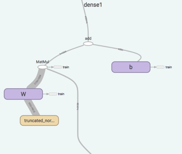
Notice the size of the output - 1024. This will be the number of neurons in the second fully connected layer. Before we get to the next layer, however, we apply the dropout technique.
h_pool2_flat = tf.reshape(h_pool2, [-1, 7*7*64])
h_fc1 = tf.nn.relu(dense_layer(h_pool2_flat, 7*7*64, 1024, "dense1"))
Dropout
Dropout is a regularization technique which controls overfitting. During the training phase, a fixed proportion of randomly selected neurons are disabled. In this example, we use a value of 0.5 to be injected into a placeholder when the network is running. So, in every iteration during training, half the neurons per layer are disabled. Note that this is only done during training and not when generating predictions on a test set.
def dropout(inp, keep_prob, name="dropout"):
   """Apply dropout with probability defined by placeholder tensor keep_prob."""
   with tf.name_scope(name):
       return tf.nn.dropout(inp, keep_prob)
keep_prob = tf.placeholder(tf.float32)
h_fc1_drop = dropout(h_fc1, keep_prob)
Create the second dense layer
Set the output size for the final fully connected layer to equal the number of classes, which is 10 for the MNIST dataset.
y_conv = dense_layer(h_fc1_drop, 1024, 10, "dense2")
We want each of the 10 neurons to output a probability. We can apply the softmax activation function to do this. In order to evaluate the model, we will also need a cost function. For classification problems, a frequent choice is cross-entropy. TensorFlow has a function that will perform both these operations in a way that is numerically stable.
As in, the functions we created for each of the layers, we use name scopes so that TensorFlow groups all the ops in the with block inside the computational graph. This helps keep the graph looking nice and clean. You can try creating a graph without the name scopes, just to get a visual on how it looks.
with tf.name_scope("xentropy"):
   cross_entropy = tf.reduce_mean(tf.nn.softmax_cross_entropy_with_logits(labels=y_, logits=y_conv))
Let's use the Adam optimizer to minimize the loss function. You might want to consider picking a learning rate with a smaller value, such as 1e-4. This is another important hyperparameter to tune - a value that is too small will require unnecessarily long training times, but a value that is too large may not achieve an optimal local minimum for the cross-entropy loss function.
lr=1e-2 # Learning rate
with tf.name_scope("train"):
   optimizer = tf.train.AdamOptimizer(learning_rate=lr)
   training_op = optimizer.minimize(cross_entropy)
We'll execute the training_op variable in the TensorFlow session. We'll also create an operation to compute the accuracy of our model.
with tf.name_scope("accuracy"):
   correct_prediction = tf.equal(tf.argmax(y_conv, 1), tf.argmax(y_, 1))
   accuracy = tf.reduce_mean(tf.cast(correct_prediction, dtype=tf.float32))
   tf.summary.scalar('accuracy', accuracy)
Create some file writers to save log data for TensorBoard to use for the visualizations.
write_op = tf.summary.merge_all()
writer_train = tf.summary.FileWriter(logdir + 'train', tf.get_default_graph())
writer_val = tf.summary.FileWriter(logdir + 'val', tf.get_default_graph())
Graph Execution
With the graph construction complete, we can now begin the execution stage. Here we create a TensorFlow session, in which we repeatedly run training_op. Even though we created variables earlier, they have to be initialized before we can actually use them. Rather than individually initializing each variable, you can use tf.global_variables_initializer(). Inside the for loop, a randomly sampled batch of 100 images is obtained from the training and validation sets. On every fifth iteration, TensorFlow writes information to disk via the write_op operation we defined earlier. Notice that we feed in the placeholders with the feed_dict argument. Once training is complete, the model is evaluated by running it on the test set. The result is then printed out to the console.
with tf.Session() as sess:
   sess.run(tf.global_variables_initializer())
   for i in range(1001):
       batch_X, batch_y = mnist.train.next_batch(100)
       val_batch_X, val_batch_y = mnist.validation.next_batch(100)
       if i % 5 == 0:
           summary_str = sess.run(write_op, feed_dict={X: batch_X, y_: batch_y, keep_prob: 1.0})
           writer_train.add_summary(summary_str, i)
           writer_train.flush()
           summary_str = sess.run(write_op, feed_dict={X: val_batch_X, y_: val_batch_y, keep_prob: 1.0})
           writer_val.add_summary(summary_str, i)
           writer_val.flush()
       training_op.run(feed_dict={X: batch_X, y_: batch_y, keep_prob: 0.5})

   test_accuracy = accuracy.eval(feed_dict={X: mnist.test.images, y_: mnist.test.labels, keep_prob:1.0})

   print('Test accuracy {}'.format(test_accuracy))
TensorBoard visualization
While the graph is executing, you can observe its progress through the TensorBoard interface. You should see some visualizations that look something like the following:
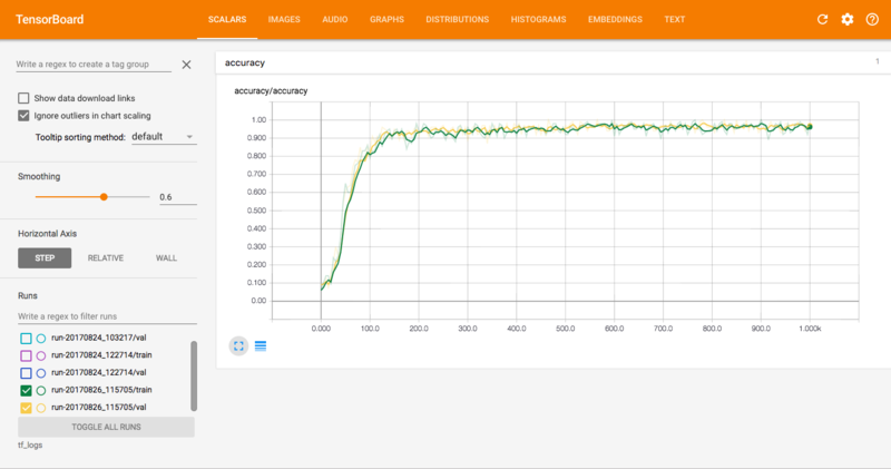
This is perhaps the most important graph. It shows the classification accuracy of the training set (green) and validation set (yellow). In general, we want the training and validation accuracies to track each other fairly closely. The gap between the training and validation accuracy shows how much your model is overfitting - if the training accuracy is higher than the validation accuracy, that means your model is overfitting. On the other hand, it is possible that the model is underfitting if the accuracies are too close - this would mean that the model is too simple to capture the complexity of the data.
For simplicity, the accuracy here is plotted against the number of iterations, but normally we would place the number of epochs on the x-axis. Check this out for more info.
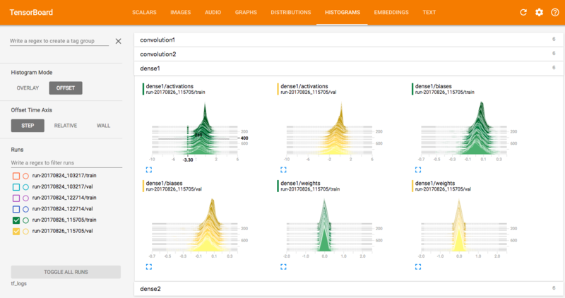
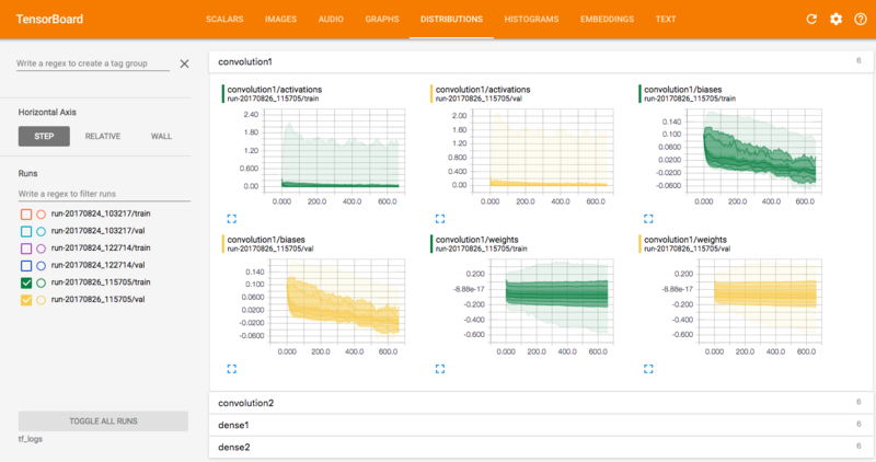
Other useful visualizations to look at are the distributions and histograms of the parameters and the activations for each layer of the network. The distribution and histogram plots essentially give you two different ways of visualizing the same thing - the distribution of parameters evolving over time. For example, in the top right graph above (the dense1 layer biases), you can see the variance increasing over time, whereas the mean is decreasing, indicated by the distribution shifting slightly to the left.
You can use these plots to diagnose problems such as an incorrect initialization of parameters in your model. Watch out for distributions getting stuck at 0 or at the extreme ends of the range of the activation function (in the case of bounded activations).
Want to learn more about TensorBoard? We found this YouTube presentation super insightful.
Conclusion
Congrats! Now you have a complete computational graph in Tensorflow! Take your time exploring the graph in TensorBoard, expanding the nodes by clicking on the plus icon in the top right-hand corner. There was some nodes we didn't get a chance to look at, such as the cross-entropy and accuracy nodes. Here is an incredibly cool visualisation of using a Neural Network (Interactive example). Try to determine some details about the network through visual inspection. What are the similarities and differences compared to the network we created in this tutorial? (Hint: some questions you could ask yourself are, "What is the size of the convolutional filter in each neural network?", "How many convolutional layers are there in each neural network?" or "What is the number of filters in each convolutional layer?")
TensorFlow's documentation is jam packed with operations, so make sure to have a read there if you want to see what functionality you can use for your next ML model.
Final Notes
Recommended product: Coding Essentials Guidebook for Developers
