How self-driving cars learn to drive

ADVERTISEMENT
Table of Contents
- Introduction
- Record data about the environment
- Analyze and process data
- Develop a model that understands the environment
- Train a model that knows how to drive
- Refine a model that improves over time
- Conclusion
Introduction
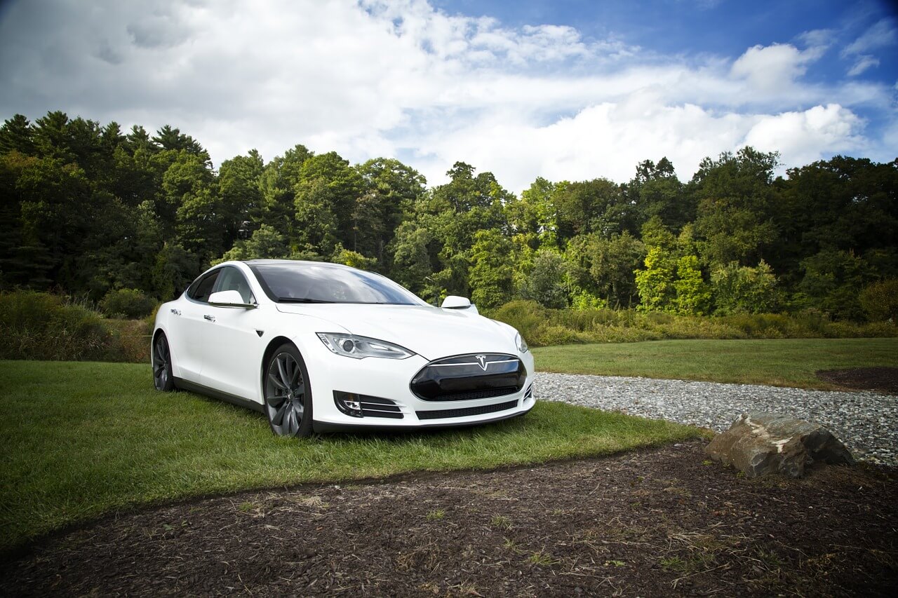
Self-driving cars took the spotlight when Tesla announced that the Model S received a 5 star safety rating after independent testing by the National Highway Traffic Safety Administration (NHTSA). You may have also seen the video of a Tesla driving autonomously. Similar to the way humans use our eyes to see the road and hands to turn the steering wheel, self-driving cars use an array of cameras to perceive the environment and a deep learning model for steering. In this article, we will cover how self-driving cars:
- Record data about the environment
- Analyze and process data
- Develop a model that understands the environment
- Train a model that knows how to drive
- Refine a model that improves over time
Record data about the environment
The first step is to record data of the car driving in different conditions. Concretely, our goal is to get a symmetrical distribution of positive and negative steering angles. We achieve this by making laps around the track, driving in both a clockwise and anti-clockwise direction. This helps to reduce turn bias, which is the tendency for the car to drift to one side of the road over time. Be mindful to drive safely at all times, as errant driving behavior may cause the model to perform poorly when we switch to autopilot. Driving at a slow speed, e.g. 10 miles per hour, also helps in logging smooth steering angles while navigating turns. Driving behaviors are categorized into:
- Driving straight:
0 <= X < 0.2 - Navigating slight turns:
0.2 <= X < 0.4 - Navigating sharp turns:
X >= 0.4 - Recovering back to the center
The formula for computing the steering angle is X = 1 / r, where X is the steering angle and r is the turning radius in meters. The fourth category "Recovering back to the center" is crucial during the data recording process. It allows the car to learn how to steer back to the center when it is about to hit a kerb or go off road. Recorded data is saved in driving_log.csv, where each row contains:
- File path to front center camera image
- File path to front left camera image
- File path to front right camera image
- Steering angle
Record about 100,000 steering angles and images, so as to provide sufficient data for training the model. Insufficient data samples may cause overfitting. Check that we have a symmetrical distribution of steering angles by plotting steering angle histograms regularly during the data recording process.
Analyze and process data
The second step is to analyze and prepare the recorded data for modeling. Concretely, our goal is to generate more training samples for the model. The image below is taken by the front center camera. It measures 320 by 160 pixels and contains red, green, and blue channels. We represent this in Python as a 3 dimensional array, where each pixel corresponds to a value from 0 to 255. We are interested in the area below the horizon and the lane markers on each side. We will use Cropping2D in Keras, an open source deep learning library, to crop the image in the third step, so as to reduce the amount of noise that is feed into the model. Keras is a useful library as it abstracts away a lot of complexity from the TensorFlow backend.
We use OpenCV, an open source computer vision library, to read an image from file and flip it along the vertical axis to generate a new sample. OpenCV is a great fit for our self-driving car use case as it is written in C++. Other image augmentation techniques, such as skewing and rotating, are also useful for generating more training samples.
center_image = cv2.imread(batch_sample[0].strip())
flip_center_image = cv2.flip(center_image, 1)
We also need to flip its corresponding steering angle by multiplying by -1.0.
flip_center_angle = transform_angle(center_angle * -1.0)
We then use Numpy, an open source library for scientific computing, to reshape the image into a 3 dimensional array that is ready for modeling.
def transform_image(image):
    IMAGE_WIDTH = 160
    IMAGE_LENGTH = 320
    IMAGE_DEPTH = 3

    image = np.array(image, dtype = 'float32')

    return image.reshape(
        IMAGE_WIDTH,
        IMAGE_LENGTH,
        IMAGE_DEPTH
    )
Develop a model that understands the environment
The third step is to design a deep learning model that extracts features from the images that we recorded. Concretely, the goal is to map an input image containing 153,600 pixels to an output containing a single float value. We implement the NVIDIA model as our base architecture. Each layer provides specific functionality that is crucial for each training epoch:
Normalize the 3 dimensional array to unit length, so as to prevent large values from skewing the weights in the model. We divide by 255.0 as that is the largest possible value that a pixel can have.
model.add(Lambda(
    lambda x: x / 255.0 - 0.5,
    input_shape = (IMAGE_WIDTH, IMAGE_LENGTH, IMAGE_DEPTH)
))
Crop pixels above the horizon and below the front of the car, so as to reduce noise.
CROP_TOP = 70
CROP_BOTTOM = 25
model.add(Cropping2D(cropping = ((CROP_TOP, CROP_BOTTOM), (0, 0))))
Convolve the 3 dimensional array to extract key features, e.g. lane markings, kerbs. This information is crucial for predicting steering angles.
model.add(Convolution2D(
    convolution_filter,
    kernel_size,
    kernel_size,
    border_mode = 'valid',
    subsample = (stride_size, stride_size),
    activation = 'relu'
))
Use dropout to reduce overfitting. We want to develop a model that can drive on any road, not just the track that we trained on.
DROPOUT = 0.2
model.add(Dropout(DROPOUT))
Output steering angle as a float. This is the single value that is sent to the Controller Area Network, which allows the model to steer the car.
model.add(Dense(1))
Train a model that knows how to drive
The fourth step is to train the model to drive on its own. Concretely, our goal is to minimize loss when predicting steering angles. We define loss as the mean square error between the predicted and actual steering angle. Keys steps in the training process:
Shuffle samples from driving_log.csv to reduce order bias.
shuffle(samples)
Split samples into a 80 % training set and 20 % validation set. This allows us to see how accurate the model is at predicting steering angles.
train_set, validation_set = train_test_split(
    samples,
    test_size = VALIDATION_SET_SIZE
)
Use Adaptive Moment Estimation (Adam) optimizer to minimize mean squared error. The key advantage of using Adam, compared to gradient descent, is using momentum to converge at an optimum value.
adam = Adam(lr = LEARNING_RATE)
model.compile(optimizer = adam, loss = 'mse')
Use a generator to fit the model. Due to the sheer number of images, it is not feasible to fit the entire training set into memory. Therefore, we use a generator to yield images in batches for training.
history = model.fit_generator(
    train_generator,
    samples_per_epoch = samples_per_epoch,
    nb_epoch = EPOCH,
    verbose = VERBOSITY,
    callbacks = callbacks,
    validation_data = validation_generator,
    nb_val_samples = validation_samples
)
Refine a model that improves over time
The fifth and final step is to refine the model, so that its accuracy and robustness improves over time. Experiment with different architectures and hyperparameters to see their effect on reducing mean square error. There is no model answer, as most refinements involve some kind of trade-off. Examples include:
- Reduce training time by using better graphics processing units (GPU) at the expense of increased cost
- Increase the probability of converging at the optimum value by lowering the learning rate at the expense of training time
- Reduce training time by using grayscale images at the expense of losing color information provided by red, green, and blue channels
- Improve gradient estimation accuracy by using a large batch size at the expense of memory usage
- Use a large number of samples per epoch to decrease loss fluctuation
Conclusion
Developing a self-driving car gives us insights into the advantages and limitations of computer vision and deep learning. We have shown how we can use both concepts to drive a car autonomously around a track. From a safety perspective, this reduces the number of accidents caused by errant driving behavior. However, we also wish to highlight that there are still edge cases in self-driving car technology that are being worked on. With companies like Tesla leading the way in innovation, we posit that self-driving cars are the future.
Final Notes
Recommended product: Coding Essentials Guidebook for Developers


